A very, very basic neural network in Python
When I first started learning about generalized linear models and optimization, my PI advised me to try implementing my own examples from scratch. I found this approach very helpful and have since started using this approach to try to gain a better understand of how a number of different aspects of machine learning work. We have so many powerful libraries for machine learning these days that sometimes you can get by with just a surface level understanding of how things work. There’s nothing wrong with that, but I sometimes get hung up when I don’t understand the details of how something works. Here, I’ve adapted an exercise from an excellent post by Andrew Trask on a toy example of a neural network implemented from scratch with Python.
Task
In this example, we are training a neural network to make a binary prediction (\(\{0,1\}\)) based on a binary input vector of size \(3\). The training data provided is:
| Inputs | Output | ||
|---|---|---|---|
| 0 | 0 | 1 | 0 |
| 1 | 1 | 1 | 1 |
| 1 | 0 | 1 | 1 |
| 0 | 1 | 1 | 0 |
From looking at this table, one might notice a pattern - the output is 1 whenever the first value in the input vector is also 1, suggesting a correlation between these two values. By training a neural network, it should also be able to learn this pattern.
The neural network architecture
Our simple neural network will sipmly pass the inputs through a single neuron with a sigmoid activation function to return an output between 0 and 11. The neural network architecture can be visualized as follows:
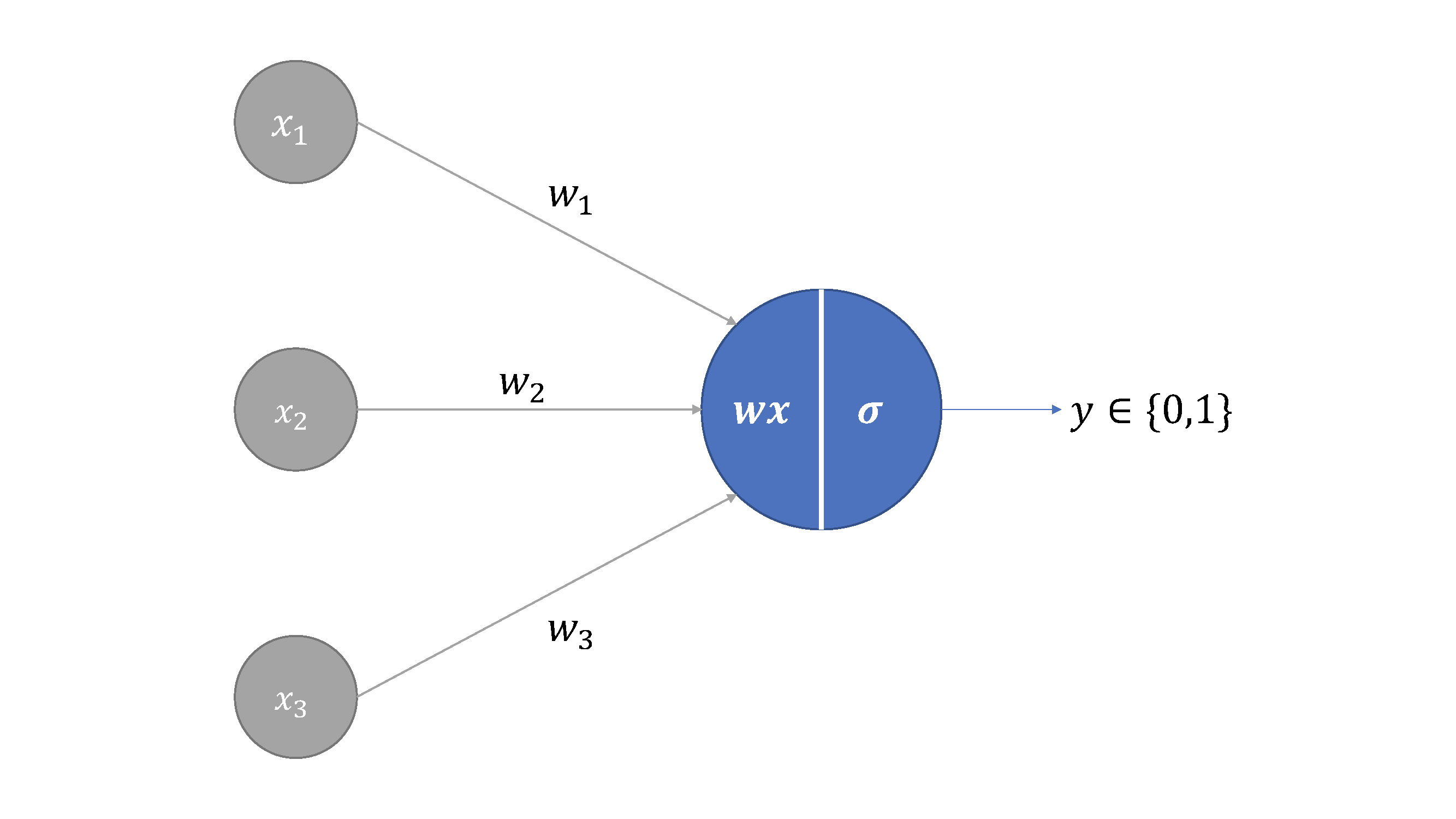
The first layer is the input channel, where each of the values in the input vector are fed into the neural network, and the second layer produces the output based on a transformation of the inputs.
Training the neural network
To train the neural network, we will use every data point (row) in the data table and pass it through the network forwards and backwards \(n\) times. Over each pass, or iteration, we will update the weights in the neural network with the goal of improving the outputs at each iteration.
Forward propagation
During forward propagation, each input row of our table (corresponds to one sample data point) will be passed through the first layer and multiplied by the hidden weights in the network via a dot product. There is a different weight for each input, producing a weighted sum:
\[s = \Sigma w_i x_i = w_1 x_1 + w_2 x_2 + w_3 x_3\]This weighted sum is then passed to a sigmoid activation function to output a prediction, \(\hat{y} = \sigma(s)\). We will repeat this for \(n\) trianing iterations.
Initializing the weights
The weights are the parameters of our neural network which we will be tuning over the course of training to try to get the most accurate predictions possible. We will start by initializing these with very small values (for simplicity’s sake, we will generate random values with a mean of 0).
Activation function
As aforementioned we will be using a sigmoid activation function, which is defined as:
\[\sigma(x) = \frac{1}{1+e^{-x}}\]Sigmoid functions are popular in machine learning because they yield an output between 0 and 1 and are also easily differentiable as:
\[\sigma ^\prime (x) = x(1-x)\]The derivative is important for the backpropgation step of this neural network, which is the step that actually helps us update the weights in each iteration of the training process.
Back propagation
This is the part where we work backwards from the predicted output of the neural network to update the weights.
Calculating the error
After each forward pass through the network, we will get a prediction for each sample in the training data from the sigmoid function. From this, we can measure the error of the prediction given the current weights as the different between the prediction and the true output value and then use this information to update the weights. In machine learning, there are various different cost functions for measuring the difference between true and predicted values. While the original blog post simply refers to the error as the difference between the true and predicted outputs, I will use a squared error cost function and demonstrate further along this post why these approaches are equivalent. The squared error cost function I will use is expressed as:
\[E = \frac{1}{2}(y-\hat{y})^2\]Here, \(y\) represents the true output while \(\hat{y}\) is the predicted output for a given training iteraction. In a more sophisticated neural network with multiple output channels, the error would be summed across all outputs, but our neural network only has one output so the expression is simpler. We add \(\frac{1}{2}\) to the beginning of this function because this function will be differentiated and the fraction allows the exponent to be canceled when differentiated. Because the derivative is typically multiplied by a learning rate anyways, it doesn’t matter that a constant is introduced here.
Updating the weights - gradient descent
The magnitude of the error from the cost function will let us know how we should adjust the current weights in the network to achieve more accurate predictions. That is, we want to adjust the weights, \(\mathbf{w}\), in response to the error, \(E\). Essentially, we’re asking the question: how does the error change as the weights change? The mathematical of this expression is \(\frac{ \partial{E} }{ \partial{w_i} }\), or the partial derivative of \(E\) with respect to a given weight \(w_i\). We can calculate this using a method called gradient descent. Gradient descent follows the curve of a function to find the set of inputs that yields the minimum output of the function. In our case, we are following the curve of the cost function to find the weights that yield the minimum error! Gradient is another way of referring to the derivative of a function - it follows that gradient descent is executed using derivatives.
Example
To get a clearer idea of how gradient descent works, we will walk through the process of updating a single weight, \(w_1\), in our model. In order to do this, we need to find all of the intermediate functions that relate \(E\) to \(w_1\). It might be easier if we visualize this:
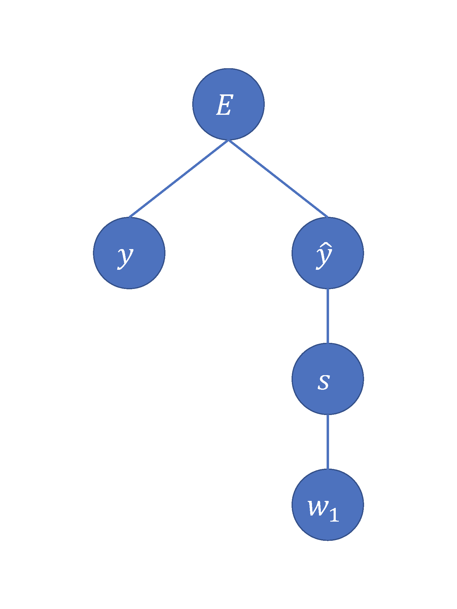
We know that the cost function is calculated from \(y\) and \(\hat{y}\), that \(hat{y}\) is calculated as \(\sigma(s)\), and that \(s\) is simply the weighted sum of the inputs and the weights \(w_1 x_1 + w_2 x_2 + w_3 x_3\). Now we have all of the functions that relate \(E\) and \(w_1\)! The reason why we want all of the intermediate functions is because we will be using the chain rule (from calculus) to calculate \(\frac{\partial{E}}{\partial{w_1}}\):
\[\frac{\partial{E}}{\partial{w_1}} = \frac{\partial{E}}{\partial{\hat{y}}} \frac{\partial{\hat{y}}}{\partial{s}} \frac{\partial{s}}{\partial{w_1}}\]The chain rule essentially breaks things down into a product of the partial derivatives of all of the intermediate functions relating \(E\) to \(w_1\).
The partial derivative of \(E\) with respect to \(\hat{y}\) is:
\[\frac{\partial{E}}{\partial{\hat{y}}} = 2*\frac{1}{2}(y-\hat{y})^{2-1}*-1 = \hat{y}-y\]The partial derivative of \(\hat{y}\) with respect to \(s\) is:
\[\frac{\partial{\hat{y}}}{\partial{s}} = \sigma ^\prime (\hat{y}) = \hat{y}(1-\hat{y})\]Finally, the partial derivative of \(s\) with respect to \(w_1\) is:
\[\frac{\partial{s}}{\partial{w_1}}=x_1+0+0 = x_1\]Therefore, for a given training iteration \(j\), we will generate an updated value of \(w_{1_{j+1}}\) by subtracting \(\frac{\partial{E}}{\partial{w_1}}\) from the value of \(w_1\) in the current iteration (\(w_{1_j}\)). This is because moving in the opposite direction of the gradient of the error will help us reach a minimum error. By extension, the value of \(\frac{\partial{E}}{\partial{w_i}}\) is the quantity by which we update any given weight \(w_i\). Typically in gradient descent, the gradient will also be multiplied by a carefully chosen step size, or learning rate, \(\eta\), but for the purpose of our example we will use \(\eta=1\). This will end up working out fine for our example, but it may not be the best learning rate for more complicated tasks and datasets.
Revisiting the original example
In Andrew Trask’s original post, he updates the weights according to the formula: \(input * error * output(1-output)\). We can see that this expression is equivalent to the expression we have derived using gradient descent. The \(input\) in his expresison is equivalent to \(x_i\) in ours; he defined \(error\) as the difference between the true and predicted outputs, or \(\hat{y}-y\) in ours; and \(output\) in his expression is simply \(\hat{y}\) in ours. I was originally confused by where his formula for updating the weights came from, so I wanted to sit down and really prove where it came from to make sure I understood. Hope this helps someone else out there too!
Summing over a batch
During each iteration of our training loop, we will evaluate all four samples (this is known as batch gradient descent). How do we integrate data from the four samples in one batch to make a single update to each value of \(w\)? For a given weight \(w_i\), an input value at the corresponding position \(x_i\) will yield a different value of \(\frac{\partial{E}}{\partial{w_i}}\) for updating the weights. We will simply sum the values obtained across all samples for each \(w_{i_j}\) to obtain a single update quantity \(w_{i_{j+1}}\). We will implement this in the code with vectorization.
Implementation
Here is the code! We will work on implementing this simple neural network with the provided training data using only numpy (and matplotlib for visualization). This tutorial can also be found as a Jupyter notebook on GitHub.
1
2
3
4
5
6
7
8
9
10
11
12
13
14
15
16
17
18
19
20
21
22
23
24
25
26
27
28
29
30
31
32
33
34
35
36
37
38
39
40
41
42
43
44
45
46
47
48
49
50
51
52
53
54
55
56
57
58
59
60
61
62
63
64
65
66
67
68
69
70
71
72
73
74
75
76
77
78
79
80
81
82
83
84
85
86
87
88
89
90
91
92
93
94
95
  import numpy as np
 import matplotlib.pyplot as plt

 # random seed for reproducibility
 np.random.seed(1)

 # a class for the simple two-layer neural network
 class SimpleNN():
    """
    initialize a simple feed-forward two layer neural network:
    - input layer of variable size
    - output layer of fixed size (1)
    """

    def __init__(self, input_size = 3):
        """
        initialize weights in network and declare input size
        """
        self.input_size = input_size
        # random weights with mean = 0
        self.weights = 2*np.random.random((input_size,1))-1

    def __sigmoid(self, weighted_sum):
        """
        sigmoid function intended to take as input weight sum of weights and inputs
        """
        return 1/(1+np.exp(-weighted_sum))

    def __gradient(self, x):
        """
        computes derivative of sigmoid function for a given value of x
        """
        return x*(1-x)

    def __accuracy(self, pred, target):
        """
        given true and predicted outputs, calculate accuracy
        """
        # binarize predicted values
        pred_bin = np.where(pred>0.5, 1, 0)
        accuracy = (pred_bin == target).sum()/target.shape[0]
        return accuracy

    def train(self, trainX, trainY, iters = 1000, verbose = False):
        """
        function for training neural network on training data
        """
        accuracy = []

        for iter in range(iters):
            ### feed forward ###

            # calculate weighted sum
            s = np.dot(trainX, self.weights)

            # predict yhat
            yhat = self.__sigmoid(s)

            ### backprop ###

            # calculate cost function
            err = trainY - yhat

            # gradient descent
            grad = np.dot(trainX.T, (yhat - trainY)*self.__gradient(yhat))

            # update weights
            self.weights -= grad

            # calculate accuracy
            accu_iter = self.__accuracy(yhat, trainY)
            accuracy.append(accu_iter)

            if verbose:
                if iter%100 ==0 or iter==0:
                    print("iter %d" % iter)
                    print("output")
                    print(yhat)
                    print("accuracy = %.2f\n" % accu_iter)

        print("output after training:")
        print(yhat)
        self.accuracy = accuracy

    def pred(self, testX):
        """
        given a previously unseen set of input data, predict output
        """
        # calculate weighted sum of inputs and weights
        s = np.dot(testX, self.weights)

        # predict yhat
        yhat = self.__sigmoid(s)

        return yhat
We’ll start by initializing our neural network and checking out the starting weights:
1
2
3
4
  nn = SimpleNN(3)

 print("starting weights")
 print(nn.weights)
The output will look something like this:
starting weights
[[-0.16595599]
 [ 0.44064899]
 [-0.99977125]]
Now let’s load in the training data as numpy arrays:
1
2
3
4
5
6
  X = np.array([[0,0,1],
              [1,1,1],
              [1,0,1],
              [0,1,1]])

 y = np.array([[0,1,1,0]]).T
Now we’ll train the network over 1,000 training iterations!
1
  nn.train(X, y)
You’ll get an output that looks something like this:
output after training:
[[0.03178421]
 [0.97414645]
 [0.97906682]
 [0.02576499]]
What are the weights after training and how have they changed from the initial weights? We can check with the function nn.weights, which will give you something like this:
array([[ 7.26283009],
       [-0.21614618],
       [-3.41703015]])
We can see that \(w_1\) is by far larger than \(w_2\) and \(w_3\), which is in line with the relationship we observed between \(x_1\) and the output \(y\) at the beginning of this tutorial.
We can also try visualizing the accuracy over each training iteration:
1
2
3
4
  plt.plot(nn.accuracy)
 plt.xlabel('training iter')
 plt.ylabel('accuracy')
 plt.show()
You should get something that looks like this:
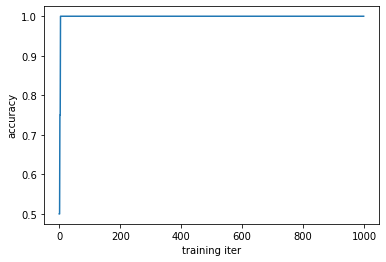
The accuracy improves pretty quickly here, likely because we have such a simple example.
Prediction
Just to make it interesting, let’s try predicting on a new data point where the input vector is \({1,0,0}\) and the corresponding true output is \(y=1\).
1
2
3
4
  testX = np.array([1,0,0])
 testY = 1

 nn.pred(testX)
If the predicted output is very close to 1, the binarizing this probability will yield a match very close to the true target value of this data point. The neural network has been trained the identify the pattern in the data and make accurate predictions!
Enjoy Reading This Article?
Here are some more articles you might like to read next: