Ordinary least squares (OLS) is a method for fitting a linear regression model using least squares - that is, minimizing the sum of the squared differences between the true vs. predicted outputs of the linear model to determine the weights that optimize the model fit. The Jupyter notebook for this tutorial can be found on my GitHub.

Simple linear regression model

A linear regression model for a sample \(i\) can be formulated as:

where \((\alpha,\beta)\) are the model parameters, \(x_i\) is a scalar predictor variable, and \(y_i\) is a response variable. \(\varepsilon_i\) is a sample specific error term.

The goal of OLS

The goal of OLS is to estimate the values of \((\alpha, \beta)\) in the model given a set of training data so as to make predictions of \(\hat{y}_i=\alpha + \beta x_i\). In order to estimate the parameter values, OLS mimizes the sum of squared errors between the observed vs. predicted response variables for each predictor $x_i$:

In the case of simple linear regression, we can estimate the parameters as follows:

Simulate data

Let’s start by simulating some data for this tutorial. We will randomly generate 100 values for each \(\mathbf{y}\) and \(\mathbf{x}\). We will also generate a residual for each value to simulate some noise (\(\varepsilon\)) in the linear relationship between \(\mathbf{x}\) and \(\mathbf{y}\). We will use predetermined values of \(\alpha = 2\) and \(\beta = 0.3\) for generating these values.

1
2
3
4
5
6
7
8
9
10
11
12
13
14
 import numpy as np
 import matplotlib.pyplot as plt
 
 # random seed
 np.random.seed(0)
 
 # define alpha and beta
 alpha = 2
 beta = 0.3
 
 # generate x, y
 x = 2 * np.random.randn(100) + 3   # generate 100 values of x with mean = 2, stddev = 3
 res = 0.5 * np.random.randn(100)   # Generate 100 error terms
 y = 2 + 0.3 * x + res   # calculate y

Estimate \(\hat{\alpha}\) and \(\hat{\beta}\)

1
2
3
4
5
6
7
8
9
 # calculate mean of x and y
 xbar = np.mean(x)
 ybar = np.mean(y)

 # estimate beta and alpha from data 
 betaHat = np.sum((x-xbar)*(y-ybar))/np.sum((x-xbar)**2)
 alphaHat = ybar - betaHat*xbar
 
 print('betaHat = %.5f, alphaHat = %.5f' % (betaHat, alphaHat))

Check and see how well these estimated values of \(\hat{\alpha}\) and \(\hat{\beta}\) match up against the values of \(\alpha=2\) and \(\beta=0.3\) that we used to generate this simulated dataset!

Predict \(\hat{\mathbf{y}}\)

Now that we have fitted our simple linear regression model, we can use the estimated parameters to make estimates of \(\hat{\mathbf{y}}\) given the predictors \(\mathbf{x}\).

1
 yhat = alphaHat + betaHat*x

Let’s plot the estimates of \(\hat{\mathbf{y}}\) against the true response variables \(\mathbf{y}\):

1
2
3
4
5
6
7
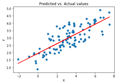
 plt.scatter(x, y)   # scatter plot showing actual data
 plt.plot(x, yhat, 'r')     # regression line
 plt.title('Predicted vs. Actual values')
 plt.xlabel('X')
 plt.ylabel('y')

 plt.show()

It should look something like this:

We can also check the Pearson correlation between \(\hat{\mathbf{y}}\) and \(\mathbf{y}\):

1
2
3
4
 from scipy.stats import pearsonr

 corr, _ = pearsonr(yhat, y)
 print("Pearson's r = %.3f" % corr)