Maximum likelihood estimation (MLE) is a method used for estimating the parameters used to define a probability distribution by fitting to observed data drawn from said distribution. As the name implies, this method involves maximizing the likelihood that the observed data comes from a statistical model. A silly analogy I sometimes use to explain MLE involves finding clothes that fit. Here, the observed data is someone who’s trying to find clothes that fit. MLE is like the process of trying on clothing items of different sizes until we find the sizes that fit the best. The clothing sizes are analogous to the parameters that define the shape of statistical distribution from which the observed data came (so the distribution itself is equivalent to the piece of clothing). Assuming the individual has no idea what their size is (this is actually somewhat realistic for womens fashion, where sizing can be wildly inconsistent across brands), MLE will start with a set of guesses at what the best sizes could be and then try different sizes to improve the fit over each iteration. In this tutorial, we will simulate data and use MLE to recover the parameters used to simulate the data. A Jupyter notebook for this tutorial can be found on my GitHub.

MLE for normally distributed data

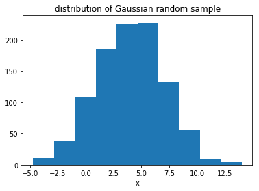
Let’s begin by walking through an example using MLE to estimate the parameters for a normal distribution from which we draw a sample set of observed data. To begin, let’s start by drawing $N=1000$ data points from a normal distribution defined as \(N(\mu=4,\sigma=3)\). We will refer to the sampled data as \(\mathbf{x} = x_1, x_2,...,x_N\).

Simulate data

1
2
3
4
5
6
7
8
9
10
11
12
13
14
15
16
17
18
 # load the packages we'll need for this tutorial
 import numpy as np
 from scipy import optimize
 from scipy import stats 
 import matplotlib.pyplot as plt
 import math
 from scipy.special import factorial
 
 # define parameters
 MU = 4
 SIGMA = 3
 N = 1000
 
 # add some noise
 noise = np.random.randn(N)
 
 # sample data from normal distribution
 norm_sample = stats.norm.rvs(loc = MU, scale = SIGMA, size = N) + noise

Visualize

Let’s take a look at what our sample data looks like.

1
2
3
4
 plt.hist(norm_sample)
 plt.xlabel('x')
 plt.title('distribution of Gaussian random sample')
 plt.show()

You should get something that looks like this:

Define likelihood function

In MLE, we want to optimize a likelihood function, which measures the likelihood that a given set of data came from a statistical distribution defined by a current set of parameters. The likelihood function (\(\mathcal{L}\) for a continuous distribution (our data is continuous) is defined as:

Here, \(\theta={\theta_1,...,\theta_M}\) represents the set of \(M\) parameters defining the distribution that we are trying to fit the data to. \(f_{\theta}(\mathbf{x})=P_{\theta}(X=\mathbf{x})\) is just another way of writing the probability density function (PDF) for the continuous distribution given the parameterization \(\theta\). In other words, it means “what is the probability that the data we are observing came from the statistical distribution defined the parameters \(\theta\)?” Now because in MLE we are typically looking at a set of data points, we are actually trying to find the joint probability that all of the data points in our sample came from the same distribution defined by a given set of parameters \(\theta\). Because the joint probability of identical and independently distributed variables is simply their product, our likelihood function can therefore be expressed as:

In our example, we will try to fit the data back to a normal distribution. Therefore, \(\theta=[\mu,\sigma]\). Even if we didn’t have the prior knowledge that we sampled our data from a normal distribution, observing the distribution of the data clearly indicates that the data follows a normal distribution, making it a good distribution to fit our data to. The PDF for the normal distribution is defined as:

This is the function that we will be trying to maximize. However, in practice it is more common to optimize over the log-likelihood function (LLF), because the product of many probability values can lead to floating point errors in computation. The LLF can be expressed as:

Optimize

Many built-in optimizers don’t have a maximization function, just a minimization function. Therefore, instead of maximizing the log-likelihood, we will minimize the negative log-likelihood.

1
2
3
4
5
6
7
8
9
10
11
 # define neg llf
 def ll_norm(params, x):
     '''
     params is a list of parameters to estimate: [mu, sigma]
     x is list of normally distributed values described by estimated params
     '''
    
     mu = params[0]
     sigma = params[1]
     loglik = np.log((1/((2*math.pi*sigma**2)**0.5))*np.exp(-((x-mu)**2)/(2*sigma**2)))
     return -loglik.sum()

Here’s a quick intro to essential arguments for the scipy.optimize.minimize function: -fun: function to minimize - for us this is the negative log-likelihood function

• x0: initia guesses for the parameters we’re estimating, in the form of a list, tuple, or numpy array
• args: any other variables to pass to the function fun, given in a list, tuple, or numpy array
• bounds: bounds for parameters to be estimated, given as a list of lists or tuple of tuples, corresponds to params in x0

1
2
3
4
5
6
7
# minimize negative log-likelihood
 norm_res = optimize.minimize(fun = ll_norm,
               x0 = [0,1],
               args = (norm_sample),
             bounds = ((None,None),(1e-6,None)))

 norm_res

The output should look something like this:

      fun: 2509.8651698184385
 hess_inv: <2x2 LbfgsInvHessProduct with dtype=float64>
      jac: array([ 0.00040927, -0.00027285])
  message: b'CONVERGENCE: REL_REDUCTION_OF_F_<=_FACTR*EPSMCH'
     nfev: 45
      nit: 14
   status: 0
  success: True
        x: array([4.02069038, 2.97703045])

Here’s a brief overview of what these outputs mean:

• fun: minimum value of function at estimated parameters
• nfev: number of function evaluations
• nit: number of iterations
• success: bool - did the optimizer run into an issue?
• x: array of estimated parameters that minimize the function, corresponding to x0

We can print the final parameter estimates from MLE and see how they compare to the values we used to simulate the data that we showed the algorithm:

1
2
 print('mu = %d, sigma = %d' % (MU, SIGMA))
 print('mu_est = %.4f, sigma_est = %.4f' % (norm_res.x[0], norm_res.x[1]))

You should see that the estimated parameters \(\hat{\mu}\) and \(\hat{\sigma}\) are quite close to the true parameter values that we used to define the normal distribution from which we simulated the data points. If you refer to my Jupyter notebook, you can also see how changing the size of the data that we give to the MLE algorithm change the resulting parameter estimates.

MLE for Poisson-distributed data

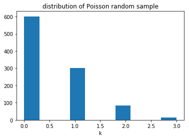
Now let’s see how we can use MLE to estimate the parameters of the distribution from which a set of Poisson distributed data came from. Poisson-distributed data is discrete and nonnegative. The Poisson distribution takes only one parameter, $\lambda>0$, which represents the rate at which events occur.

It is a discrete probability distribution that expresses the probability of a given number of events, \(k\), occurring in a fixed interval of time or space, if the events occur with a known constant rate \(\lambda\) and independently of the time since the last event.

Here, we will randomly generate a set of Poisson distributed data for a specified value of \(\lambda\).

Note: The scipy notation for the Poisson distribution uses \(\mu\) in place of \(\lambda\).

Simulate data

1
2
3
4
5
6
 # define parameters
 LAMBDA = 0.5
 N = 1000
 
 # sample data from poisson distribution
 pois_sample = stats.poisson.rvs(loc = MU, scale = SIGMA, size = N)  

Visualize

Let’s take a look at what our sample data looks like.

1
2
3
4
 plt.hist(pois_sample)
 plt.xlabel('kpois_sample')
 plt.title('distribution of Poisson random sample')
 plt.show()

You should get something that looks like this:

Define likelihood function

For a discrete distribution such as the Poisson, the likelihood function doesn’t change much, except it takes the products of the probability mass functions (PMF) rather than the probability distribution function (PDF):

or,

Again, we will need to define the PMF for the Poisson distribution to define our likelihood function. Because the Poisson is parameterized by \(\lambda\), \(\theta=[\lambda]\) for our likelihood function.

Again, we will minimize over the negative LLF. The LLF for the Poisson is expressed as:

Optimize

1
2
3
4
5
6
7
 def ll_pois(params, k):
     '''params is list of parameters to estimate: [lambda]
     k is list of Poisson distributed values described by estimated parameter'''
    
     lmbd = params[0]
     loglik = np.log(np.exp(-lmbd)*(lmbd**k)/factorial(k))
     return -loglik.sum()

Note: When you want to set bounds but you only have one parameter to estimate, you need to format it as demonstrated below, or you will run into an error.

1
2
3
4
5
6
 pois_res = optimize.minimize(fun = ll_pois,
               x0 = [1e-6],
               args = (poisson_sample),
             bounds = ((1e-6,None),))

 pois_res

The output should look something like this:

      fun: 937.3870827020155
 hess_inv: <1x1 LbfgsInvHessProduct with dtype=float64>
      jac: array([-0.0001819])
  message: b'CONVERGENCE: REL_REDUCTION_OF_F_<=_FACTR*EPSMCH'
     nfev: 56
      nit: 17
   status: 0
  success: True
        x: array([0.51099991])

We can print the coefficients:

1
2
 print('lambda = %.1f' % LAMBDA)
 print('lambda_est = %.4f' % pois_res.x[0])

scipy has built-in pdf and logpdf functions for a number of statistical distributions, so in practice you could use those functions instead of implementing them yourself.