Gradient descent
Gradient descent is an optimization algorithm used to find the optimal weights for a model. While it is popularly used to tune the weights in neural networks, in this tutorial we will be using it to try to recover the coefficients used to simulate a toy dataset. We will also demonstrate the differences between batch, stochastic, and mini-batch gradient descent and defining some of the relevant terms. Here is the link to the Jupyter notebook for this tutorial on my GitHub.
Simulating the data
We will begin by simulating the data for this example. Our simulated dataset will contain \(n=10000\) samples using a linear function defined as:
\[f(x_1, x_2, x_3) = ax_1 + bx_2 + cx_3 + \varepsilon\]Here, \({x_1,x_2,x_3}\) represent an input vector of size 3 and \(\varepsilon\) is noise.
To do this, we will first simulate the coefficients of the model, \(a,b,c\) by picking 3 random integers between 1 and 10.
1
2
3
4
5
6
7
  import numpy as np
 np.random.seed(1)

 # simulate coeffs
 coeffs = np.random.randint(1,10,size = 3)

 print("Coefficients: a = %d, b = %d, c = %d" % (coeffs[0], coeffs[1], coeffs[2]))
Next, we will generate the inputs and the noise for each sample by randomly sampling from the standard normal distribution, and then calculate the outputs based on the equation defined above.
1
2
3
4
5
6
7
8
9
10
11
  # define number of data points
 n = 10000

 # define inputs in dataset
 X = np.random.randn(n,3)

 # define noise
 noise = np.random.randn(n)

 # get outputs for dataset
 y = np.sum(X*coeffs, axis = 1) + noise
Just to get a better idea of what the data looks like, let’s coerce the dataset we’ve simulated into a data frame format and take a look at it.
1
2
3
  import pandas as pd

 pd.DataFrame(np.hstack((X, np.reshape(y, (-1,1)))), columns = ["x1","x2","x3","y"])
Now let’s cover the concepts that will be important for this tutorial.
Gradient descent
Gradient descent is an optimization method that is popularly used in machine learning to find the best parameters (more often referred to as weights in the case of neural networks) for a given model. It works quite like how it sounds - by following gradients to descend towards the minimum of a cost function. Cost functions are a function of the difference between the true and predicted outputs of a given model. There are a number of different cost functions out there. For example, cross entropy cost functions are popularly used for classification problems while squared error cost functions are popular used for regression problems. Conceptually, gradient descent looks something like this:
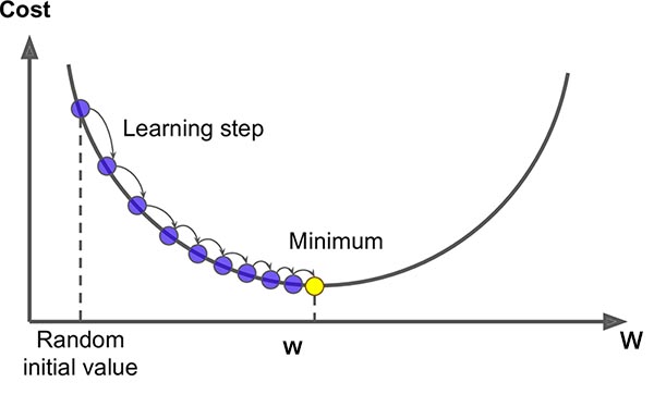
The y-axis represents the possible values of the cost function, or error, evaluated for different model weights \(\mathbf{w} = \{w_1, w_2,...,w_j\}\) where \(j\) is the total number of weights in the model. In the beginning of the model training process, we have random weight values which will yield different errors. At each iteration of training, we will calculate the gradient at the point in the cost function given the current weights, multiply the gradient by a pre-determined learning rate, and then descend along the cost function curve accordingly.
Types of gradient descent
There are a couple of different types of gradient descent out there. In order to understand the differences between these, it is first helpful to define some of the following terms:
- sample: a sample is a single data point that can be passed to the model
- batch: a hyperparameter which defines the number of samples that the model must evaluate before updating the weights in the model
- epoch: a hyperparameter that defines the number of time that the entire training dataset will be passed through the model
Now, we can start talking about the different types of gradient descent!
Batch gradient descent
In batch gradient descent, every data point in our dataset is evaluated in a given training iteration and the gradients are summed for each data point and then used to make a single update to the weights in the model. In other words, the size of a batch is equivalent to the size of the entire training data set, and the number of batches in an epoch is 1.
Pros
- Because we only update the model after evaluating all data points, this results in fewer updates and a more computationally efficient training process
- Fewer udpates results in a more stable gradient and more stable convergence
Cons
- The more stable gradient may result in the model converging earlier to a less optimal set of parameters, e.g. a local minimum instead of a global minimum
- Prediction errors must be accumulated across all training samples because the model weights are updated after evaluation of all samples
- Usually the entire dataset needs to be loaded in memory for the model to work with it
- Altogether these cons make this approach slower
Stochastic gradient descent (SGD)
In stochastic gradient descent, a random subset of the training dataset is evaluated in each training iteration to provide a single update to the weights in the model. Typically, SGD refers to a random subset size of 1; that is, each batch consists of a single sample. The number of batches in a single epoch, then, is equivalent to the number of samples in the entire training data set.
Pros
- Because the model weights are updated more frequently, we can have a higher resolution of the how the model performs and how quickly it’s learning
- The higher frequency of model updates may help the model learn faster for some problems
- The “noisier” model updates may help the model avoid local minima
Cons
- Updating the model more frequently is more computational expensive
- The more frequent model updates result in noisier gradients, resulting in more variance in the error landscape across training epochs
- The noisier updates can also make it harder for the algorithm to optimize
(Stochastic) mini-batch gradient descent
As with SGD, we are picking random subsets of the data to pass through the model in order to inform the updating of the weights; however, here the batch size is somewhere between a single sample and the entirety of the training data set. Therefore, in a single epoch we see a number of samples roughly equivalent to the total number of samples in the training dataset divided by the batch size. This is very popular for training neural networks.
Pros
- More frequency model updates than batch gradient descent allows for a more robust convergence and a better likelihood of avoiding local minima
- Less frequent model updates than SGD results in greater computational efficiency
- Smaller batches means that we don’t have to have the entire training dataset in memory (as with batch gradient descent)
Cons
- We have to define an additional batch size hyperparameter
Cost function
I will be using two closely related terms in this section: loss function and cost function. A loss function is calculated for a single data point while a cost function is the sum of the losses across all the points in a batch. For our tutorial, we will use the Least Squared Error loss function, which is commonly used for linear regression. For a given sample \(j\), it is defined as:
\[LSE = \frac{1}{2}(\hat{y}_j - y_j)^2\]where \(\hat{y}_i\) is the predicted output for a given input vector \(\mathbf{x_i}\). Its associated cost function is known as Mean Squared Error (MSE):
\[MSE = \frac{1}{2m} \sum _{j=1} ^{m} (\hat{y}_j - y_j)^2\]where \(m\) is the total number of training samples.
In our example, \(\hat{y}_j\) is calculated as a linear function that is essentially the dot product between the weights in the model, \(\mathbf{w}\) and the inputs for a given sample, \(\mathbf{x}_j\):
\[\hat{y}_j = w_1 x_{i_1} + w_2 x_{i_2} + w_3 x_{i_3}\]Thus, the cost function can be expression as a function of \(\mathbf{w}\):
\[J(\mathbf{w}) = \frac{1}{2m} \sum _{j=1} ^{m} ((w_1 x_{j_1} + w_2 x_{j_2} + w_3 x_{j_3}) - y_j)^2\]By training on the data we simulated using the coefficients \(a, b, c\), we are trying to optimize the weights \(w_1, w_2, w_3\) to try to recover the coefficients used to generate the data.
Here, let’s define the functions we’ll use for calculating \(\hat{y}_j\) and MSE:
1
2
3
4
5
6
7
8
9
10
11
12
13
14
  def pred(x, weights):
     """
     predict y given inputs and weights
     """
     y_pred = np.dot(x, weights)
     return y_pred


 def mse(y_pred, y_true, m):
     """
     calculate MSE
     """
     mse = (1/(2*m))*np.sum(np.square(y_pred - y_true))
     return mse
Learning rate
The learning rate is a small value that determines how far along the curve we move to update the weights. It’s important to pick the right learning rate - a large learning rate can result in overshotting the optimum value, while a small learning rate will make it take much longer for the model to converge on the optimum.
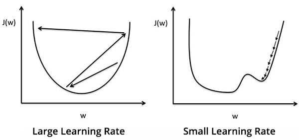
The learning rate will be denoted by \(\eta\). In our tutorial, let’s assign a learning rate of \(\eta = 0.01\).
1
2
 # learning rate
 lr = 0.01
Gradient descent algorithm
In each iteration of the training algorithm, we will update each weight in our model \(w_i \rightarrow w_i'\) with the following formula:
\[w_i' = w_i - \eta \frac{\partial{J}}{\partial{w_i}}\]where
\[\frac{\partial{J}}{\partial{w_i}} = \frac{1}{m} \sum _{j=1} ^{m} ((w_1 x_{j_1} + w_2 x_{j_2} + w_3 x_{j_3}) - y_i)(x_{j_i})\]Let’s define the function for calculating the gradient of the cost function:
1
2
3
4
5
6
  def grad(m, y_pred, y_true, x_i):
     """
     calculate the partial derivative of cost function wrt w_i
     """
     grad = (1/m) * np.sum((y_pred - y_true)*x_i)
     return grad
Now let’s begin implementing our code! We’ll start with an example of batch gradient descent.
Example - batch gradient descent
In batch gradient descent, each epoch contains only one batch, and the batch size is equivalent to the entire size of the training dataset. We will define 1000 epochs.
1
2
3
4
5
6
7
8
9
10
11
12
13
14
15
16
17
18
19
20
21
22
23
24
25
26
27
28
29
30
31
32
33
34
35
36
37
  epochs = 1000
 m = n

 # initialize random weights to start
 weights = np.random.randn(3)
 print("initial weights:")
 print(weights)

 # collect value of cost function at each iter
 cost_list = []

 # collect the weights at the end of each epoch
 weights_updates = np.zeros((epochs+1, 3))
 weights_updates[0,:] = weights

 start = time.time()
 for iter in range(epochs):
     print('epoch = %d' % iter)

     # predict on training set
     y_pred = np.apply_along_axis(pred, 1, arr = X, weights = weights)

     # calculate cost
     cost = mse(y_pred, y, m)
     cost_list.append(cost)

     # update the weights
     for i in range(weights.shape[0]):
         weights[i] = weights[i] - lr*grad(m, y_pred, y, X[:,i])

     print(weights)
     weights_updates[iter+1, :] = weights

 end = time.time()

 # calculate time
 batch_gd_time = end - start
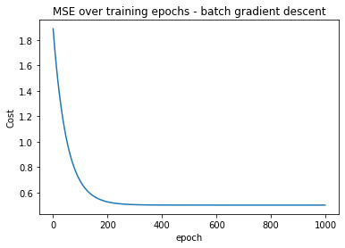
Let’s visualize the MSE over each training iteration:
1
2
3
4
5
  plt.plot(cost_list)
 plt.ylabel("Cost")
 plt.xlabel("epoch")
 plt.title("MSE over training epochs - batch gradient descent")
 plt.show()
You should see something like this:
Let’s also visualize how the weights changed at the end of each training epoch:
1
2
3
4
5
6
7
8
  plt.plot(weights_updates[:,0], label = "w1")
 plt.plot(weights_updates[:,1], label = "w2")
 plt.plot(weights_updates[:,2], label = "w3")
 plt.legend()
 plt.ylabel('weights')
 plt.xlabel("epochs")
 plt.title("Weights over training epochs - batch gradient descent")
 plt.show()
You should see something like this:
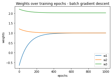
Now let’s examine weights. It should be a numpy array that contains values that look something like this:
array([1.00021995, 1.00020721, 2.02081245])
Out of curiosity, let’s run linear regression on our data and see how the coefficients obtained with the regression compare to what we got with our implementation of gradient descent.
1
2
3
4
  from sklearn.linear_model import LinearRegression

 reg = LinearRegression().fit(X, y)
 reg.coef_
The resulting coefficients probably look something like this:
array([1.00032104, 1.00020243, 2.02069302])
If we compare them to the coefficients we used to simulate this dataset, we can see that they are indeed very close to one another!
1
2
  model_results = pd.DataFrame(np.array([weights, reg.coef_, coeffs]).transpose(), columns = ['batch gradient descent','linear regression','true coeffs'])
 model_results
| index | batch gradient descent | linear regression | true coeffs |
|---|---|---|---|
| 0 | 1.0002417538638582 | 1.0003210378934184 | 1.0 |
| 1 | 1.000179104020437 | 1.000202425f449444 | 1.0 |
| 2 | 2.0206704597237226 | 2.020693020186785 | 2.0 |
Example - SGD
Now we’ll implement SGD. We will adapt the code from earlier, except now each batch is of size 1 (\(m=1\)).
1
2
3
4
5
6
7
8
9
10
11
12
13
14
15
16
17
18
19
20
21
22
23
24
25
26
27
28
29
30
31
32
33
34
35
36
37
38
39
  # define batch size
 m = 1

 # reinitialize weights
 weights = np.random.randn(3)

 # collect avg cost at each epoch
 avg_cost_list = []

 # collect the updated weights at each epoch
 weights_updates = np.zeros((epochs+1, 3))
 weights_updates[0,:] = weights

 start = time.time()
 for iter in range(epochs):
     print('epoch = %d' % iter)

     # collect losses for every batch in epoch
     epoch_loss = []

     for batch in range(X.shape[0]//m):
         # predict on training set
         y_pred = pred(X[batch,:], weights)

         # calculate cost
         cost = mse(y_pred, y[batch], m)
         epoch_loss.append(cost)

         # update the weights
         for i in range(weights.shape[0]):
             weights[i] = weights[i] - lr*grad(m, y_pred, y[batch], X[batch,i])

     # save avg cost for epoch across all batches
     avg_cost_list.append(np.average(epoch_loss))
     weights_updates[iter+1,:] = weights

 end = time.time()

 sgd_time = end - start
Now let’s plot the avefrage MSE across each training epoch:
1
2
3
4
5
  plt.plot(avg_cost_list)
 plt.ylabel("Avg. cost")
 plt.xlabel("epoch")
 plt.title("Avg. MSE over training epochs - SGD")
 plt.show()
You should see something like this:

We’ll also plot how the weights changed after each training epoch:
1
2
3
4
5
6
7
8
  plt.plot(weights_updates[:,0], label = "w1")
 plt.plot(weights_updates[:,1], label = "w2")
 plt.plot(weights_updates[:,2], label = "w3")
 plt.ylabel('weights')
 plt.xlabel("epoch")
 plt.legend()
 plt.title("Weights over training epochs - SGD")
 plt.show()
You should see something like this:

In the previous example of batch gradient descent, it looked like our model began to converge around 200 training epochs. Here, because we updated the model weights after evaluating each sample, we appear to have actually minimized the cost very early on in the training process. However, the weights that the model has converged on seem to be slightly less accurate compared to batch gradient descent. Let’s add these results to the data frame and take a look:
1
2
  model_results['SGD'] = weights
 model_results
| index | batch gradient descent | linear regression | true coeffs | SGD | mini-batch |
|---|---|---|---|---|---|
| 0 | 1.0002417538638582 | 1.0003210378934184 | 1.0 | 1.1791146471366072 | 0.9970121830081912 |
| 1 | 1.000179104020437 | 1.000202425449444 | 1.0 | 1.0082643415913106 | 1.0008372545371162 |
| 2 | 2.0206704597237226 | 2.020693020186785 | 2.0 | 1.9850734474472451 | 2.0208606244363096 |
Example - mini-batch stochastic gradient descent
Now let’s modify the code from the SGD example to accomodate mini-batch gradient descent. Let’s define the batch size as \(m=100\) to yield 100 batches per epoch. First we’ll define a function for partioning our data into batches:
1
2
3
4
5
6
7
8
9
10
11
12
13
14
15
16
17
  def batch(X, y, batch_size):
     '''
     code for partitioning dataset into batcehs
     '''

     # shuffle indices of samples
     sample_ix = np.arange(n)
     np.random.shuffle(sample_ix)

     batches = []

     for batch_ix in range(n//m):
         # determine which samples to pick for batch
         samples_in_batch = sample_ix[batch_ix*m:(batch_ix*m + m )]
         batches.append([X[samples_in_batch,:], y[samples_in_batch]])

     return batches
Now we’ll modify the code from our SGD example to implement mini-batch gradient descent:
1
2
3
4
5
6
7
8
9
10
11
12
13
14
15
16
17
18
19
20
21
22
23
24
25
26
27
28
29
30
31
32
33
34
35
36
37
38
39
40
41
42
43
44
45
46
47
  # define batch size
 m = 100

 # reinitialize weights
 weights = np.random.randn(3)

 # collect avg cost at each epoch
 avg_cost_list = []

 # collect the updated weights at each epoch
 weights_updates = np.zeros((epochs+1, 3))
 weights_updates[0,:] = weights

 # get batched data
 batches = batch(X, y, m)

 start = time.time()

 for iter in range(epochs):
     print('epoch = %d' % iter)

     # collect losses for every batch in epoch
     epoch_loss = []

     for batch_ix in range(X.shape[0]//m):

         batch_X = batches[batch_ix][0]
         batch_y = batches[batch_ix][1]

         # predict on training set
         y_pred = pred(batch_X, weights)

         # calculate cost
         cost = mse(y_pred, batch_y, m)
         epoch_loss.append(cost)

         # update the weights
         for i in range(weights.shape[0]):
             weights[i] = weights[i] - lr*grad(m, y_pred, batch_y, batch_X[:,i])

     # save avg cost for epoch across all batches
     avg_cost_list.append(np.average(epoch_loss))
     weights_updates[iter+1,:] = weights

 end = time.time()

 minibatch_time = end - start
Now we’ll plot the average MSE at each epoch:
1
2
3
4
5
  plt.plot(avg_cost_list)
 plt.ylabel("Avg. cost")
 plt.xlabel("epoch")
 plt.title("Avg. MSE over training epochs - mini-batch gradient descent")
 plt.show()

And how the weights changed after each epoch:
1
2
3
4
5
6
7
8
  plt.plot(weights_updates[:,0], label = "w1")
 plt.plot(weights_updates[:,1], label = "w2")
 plt.plot(weights_updates[:,2], label = "w3")
 plt.ylabel('weights')
 plt.xlabel("epoch")
 plt.legend()
 plt.title("Weights over training epochs - mini-batch gradient descent")
 plt.show()

Finally, we’ll compare the results we got from batch gradient descent to the other approaches:
1
2
  model_results['mini-batch'] = weights
 model_results
| index | batch gradient descent | linear regression | true coeffs | SGD | mini-batch |
|---|---|---|---|---|---|
| 0 | 1.0002417538638582 | 1.0003210378934184 | 1.0 | 1.1791146471366072 | 0.9970121830081912 |
| 1 | 1.000179104020437 | 1.000202425449444 | 1.0 | 1.0082643415913106 | 1.0008372545371162 |
| 2 | 2.0206704597237226 | 2.020693020186785 | 2.0 | 1.9850734474472451 | 2.0208606244363096 |
Let’s also compare the time it took to run these three different types of gradient descent:
1
2
3
  print("batch gradient descent time: %.3f" % batch_gd_time)
 print("SGD time: %.3f" % sgd_time)
 print("mini batch gradient descent time: %.3f" % minibatch_time)
This will give you something that looks like this:
batch gradient descent time: 35.231
SGD time: 517.481
mini batch gradient descent time: 6.185
Overall, all methods managed to converge on weights that are close to the true values we used to generate the data, and also comparable to the results of using sklearn’s linear regression function. However, we observed that SGD and mini-batch appeared to converge faster. Using SGD and mini-batch gradient descent, we could have probably reduced the number of epochs to reach the optimal weights in less time. SGD took very long to run because we updated the model weights after evaluating every single sample, and every single sample was evaluated 1000 times. Mini-batch gradient descent was much faster, and demonstrates that it is a good mix of the pros and cons of batch gradient descent and SGD.
Enjoy Reading This Article?
Here are some more articles you might like to read next: