Generalized linear models
Generalized linear models (GLMs) are something I’ve worked a lot with during my PhD. This tutorial is adapted from a lesson I developed for the bootcamp course I taught for first years in my PhD program. A Jupyter notebook for this tutorial can be found on my GitHub. As the name implies, GLMs are a generalized form of linear regression. Linear regression models make a number of assumptions about the data:
- there must be a linear relationship between the response variable and the predictors (linearity)
- the predictor variables, \(x\), can be treated as fixed values rather than random variables (exogeneity)
- the variance of the errors does not depend on the values of the predictorr variables, \(x\) (homoscedacity)
- the errors of the response variables, \(y\), are not correlated with one another (independence of errors)
- there does not exist a linear relationship between two or more of the predictor variables (lack of perfect multicollinearity)
Ordinary linear regression and its assumptions
Ordinary linear regression predicts the expected value of a response variable, \(y\), as a linear combination of predictors, \(\mathbf{x}\). That is, for a given data point \(i\) in a data set of size \(n\), \(\{ y_i,x_{i1}, ..., x_{ip} \} _{i=1}^{n}\), a linear regression model assumes that:
\[y_i = \beta_0 + \beta_1 x_{i1} + ... + \beta_p x_{ip} + \varepsilon _i = \mathbf{x}_i ^T \mathbf{\beta} \forall i=1,...,n\]where \(\varepsilon\) is an error term that adds noise to the linear relationship between the predictors and the response variables. This expression can also be expressed in matrix notation as
\[\mathbf{y} = \mathbf{X \beta} + \mathbf{\varepsilon}\]One of the implications of ordinary linear regression is that a constant change in the predictors leads to a constant change in the response variables (a linear-response model). However, this assumption is violated by certain types of repsonse variables. For example, when the response variable is restricted to being a positive value, or when the response variable is non-linear with relation to the predictors, or when the response is binary or categorical. Generalized linear models solve this problem by allowing for response variables that are not restricted to being normally distributed. Instead, it allows for some function of the response variable, known as the link function, to have a linear relationship with the predictors.
GLMs and link functions
In a GLM, it is assumed that each response variable \(y\) comes from some statistical distribution in the exponential family. These inclued, but are not limited to, the normal distribution. The mean, or expected value, of the response variable \(y\) given the predictors \(\mathbf{X}\) can be expressed as:
\[E(\mathbf{y}|\mathbf{X}) = \mathbf{\mu} = g^{-1}(\mathbf{X}\beta)\]Here, \(g\) is a link function that relates the linear predictor \(\mathbf{X \beta}\) to the expected value of the response variable \(y\) conditional upon the predictors \(\mathbf{X}\). The link function used depends on the distribution of the response variables you’re working with.
Load data for tutorial
In this tutorial, we will work with a dataset containing information about California standardized testing results (STAR test) for grades 2-11. This dataset is loaded with the statsmodels package and contains test results for 303 unified school districts. Here, the binary response variables respresent the number of 9th graders scoring above the national median for the math section. Notes about the data can be found at the link, or viewed with the command print(sm.datasets.star98.NOTE). Let’s break down the data:
-
NABOVEandNBELOWare the binary response variable -
LOWINCthroughPCTYRRNDare the 12 independent variables, or regressors. These would be represented by \(\mathbf X_1,...,\mathbf X_p\) for \(p\) regressors. - There are 8 interaction terms, representing non-linear interactions between two or more regressors. When an interaction is present, the effect of a regressor on the response variable depends on the value(s) of the variable(s) which it interacts with. The values of these interaction variables is simply the product of its interacting terms; for example, if variables \(A\) and \(B\) are interacting, the value of its interaction term, \(\mathbf X_{AB} = \mathbf X_A \circ \mathbf X_B\).
Now, let’s load the data as a data frame:
1
2
3
4
5
6
7
8
9
10
11
12
13

 # import packages for tutorial
 import statsmodels.api as sm
 import pandas as pd
 import numpy as np
 from scipy import stats
 import matplotlib.pyplot as plt
 import seaborn as sns
 import math
 from scipy import optimize

 # load dataset as pandas dataframe
 data = sm.datasets.star98.load_pandas()
In statsmodels, endog refers to the response variable(s). In this case, it will return the values of NABOVE and NBELOW. Running data.endog.head() should return a data frame that looks like this:
| index | NABOVE | NBELOW |
|---|---|---|
| 0 | 452.0 | 355.0 |
| 1 | 144.0 | 40.0 |
| 2 | 337.0 | 234.0 |
| 3 | 395.0 | 178.0 |
| 4 | 8.0 | 57.0 |
exog refers to all of the other independent variables/regressors/interaction terms. Running data.exog.head() should return a data frame that contains the rest of the dsata.
Visualize the data
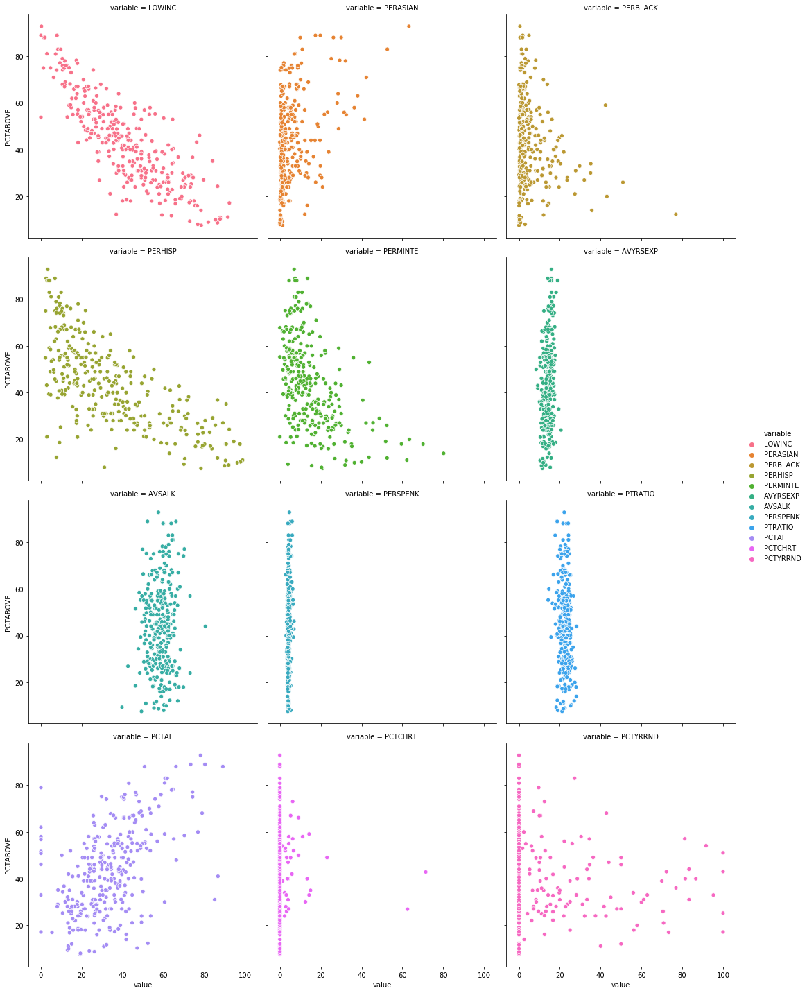
Let’s visualize the data and get a high-level idea of what’s going on. To start, let’s use seaborn to visualize the relationship between each of the independent variables (excluding the interaction terms) and the percentage of 9th grade students in each district scoring above the national median on the math section of the STAR test (100*NABOVE/(NABOVE+NBELOW)).
It will be convenient to first reformat the data table into a form that is more friendly for exploratory data visualization. If you recall, each column represents a variable. We will reshape the table such that for each of the response variables (id_vars), there is one entry for each of the regressors (value_vars). By default, any columns not set as id_vars will be interpreted as value_vars. Each sample will have a record of the variable name and value. This process is called melting the dataframe.
Here, we will subset the data table to the columns containing the binary response variables (NABOVE and NBELOW) and the first 12 variables (excluding the interaction terms). This corresponds to the first 14 columns of the dataframe.
1
2
  plot_df = data.data.iloc[:,:14].melt(id_vars = ['NABOVE','NBELOW'])
 plot_df.head()
This should return a data frame that looks something like this: |index|NABOVE|NBELOW|variable|value| |—|—|—|—|—| |0|452.0|355.0|LOWINC|34.3973| |1|144.0|40.0|LOWINC|17.36507| |2|337.0|234.0|LOWINC|32.64324| |3|395.0|178.0|LOWINC|11.90953| |4|8.0|57.0|LOWINC|36.88889|
Next, we add columns corresponding to the percentage of students above the national median (PCTABOVE) and the percentage of students below the national median (PCTBELOW).
Then we will use seaborn to generate line plots relating PCTABOVE to each of the 12 independent variables selected.
1
2
3
4
5
6
7
8
  # calculate PCTABOVE and PCTBELOW
 plot_df['PCTABOVE'] = 100*plot_df['NABOVE']/(plot_df['NABOVE']+plot_df['NBELOW'])
 plot_df['PCTBELOW'] = 100*plot_df['NBELOW']/(plot_df['NABOVE']+plot_df['NBELOW'])

 # plot
 sns.relplot(x = 'value', y = 'PCTABOVE', hue = 'variable', kind='line',
              col = 'variable', col_wrap=3, aspect=1, data = plot_df)
 plt.show()
This should give you a plot that looks like this:
We can do the same thing but with PCTBELOW on the y-axis.
1
2
3
4
 # plot
 sns.relplot(x = 'value', y = 'PCTBELOW', hue = 'variable', kind='line',
              col = 'variable', col_wrap=3, aspect=1, data = plot_df)
 plt.show()
This will give you a plot that looks like this:
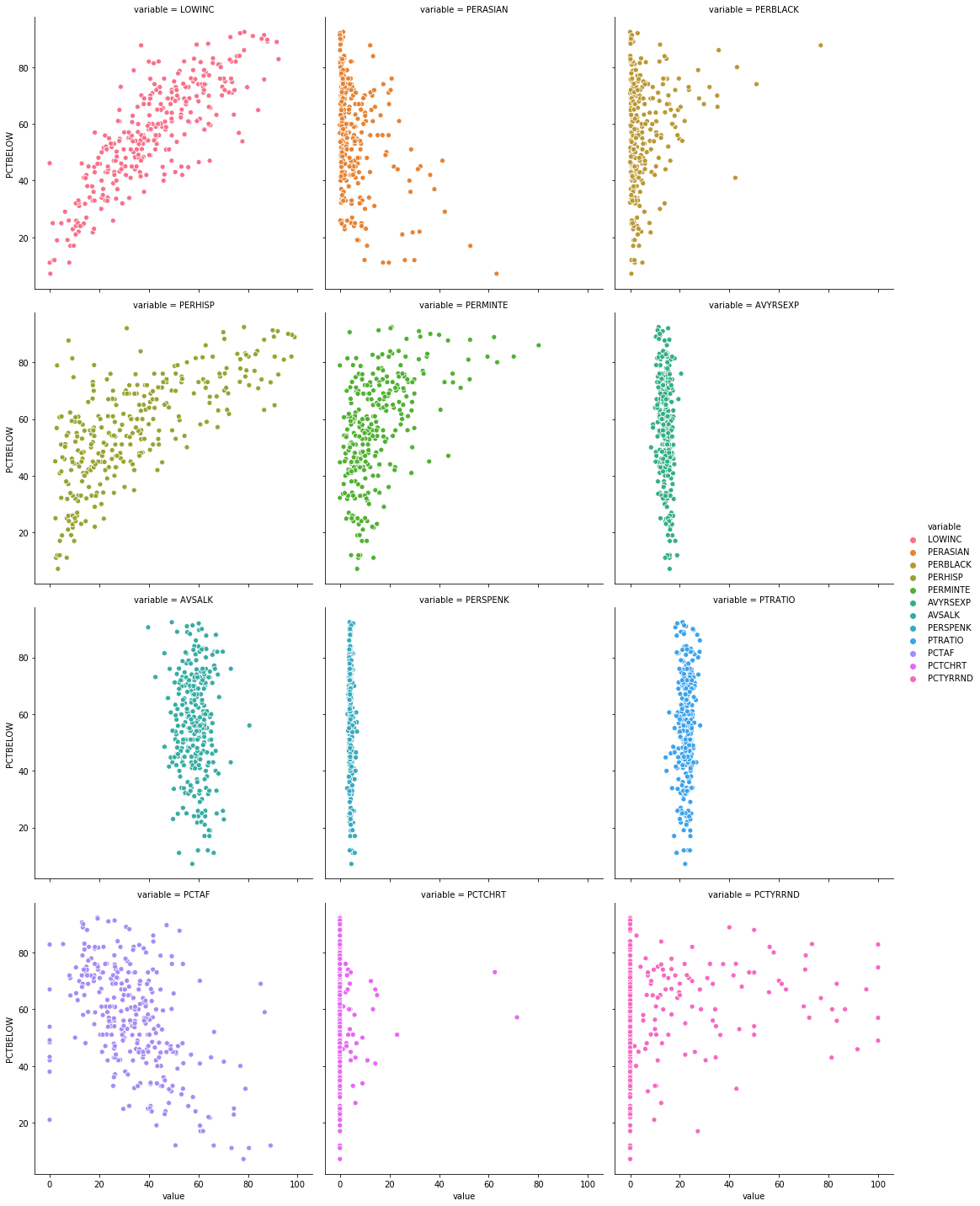
We see that the trends appear to be flipped, which is what we’d expect - variables that are positively correlated with the number of students scoring above the mean are most likely to be negatively correlated with the opposite outcome (number of students scoring below the mean).
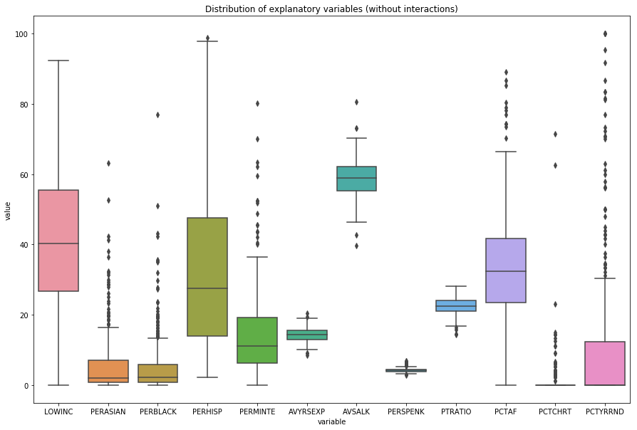
We can also take a look at hte distributions of the values of the independent variables (excluding interaction terms).
1
2
3
4
  plt.figure(figsize = (15,10))
 sns.boxplot(x='variable',y='value',data = data.exog.iloc[:,:12].melt())
 plt.title('Distribution of explanatory variables (without interactions)')
 plt.show()
This will give you a plot that looks like this:
The Binomial distribution
The response variable is binomially distributed - this means you have a discrete, non-negative number of “successes” and a discrete, non-negative number of “failures”. Here, this corresponds to NABOVE and NBELOW.
Parameterization
The binomial distribution is parameterized by \(n\in \mathbb N\) and \(p\in [0,1]\), and is expressed as \(X\sim\text{Binomial}(n,p)\), where \(X\) is a binomial random variable.
(Note: this is not the same \(p\) that we used earlier to define the dimensionality of each input vector \(\mathbf{x}_i ^T\)).
PMF
The probability mass function expresses the probability of getting \(k\) successes in \(n\) trials:
\[p(k,n,p)=\Pr(k;n,p)=\Pr(X=k)={n\choose k}p^k(1-p)^{n-k}\]for \(k=0,1,2,...,n\) where \({n\choose k}\) is the binomial coefficient:
\[{n\choose k}=\frac{n!}{k!(n-k)!}\]Essentially:
- \(k\) successes occur with probability \(p^k\), and
- \(n-k\) failures occur with probability \((1-p)^{n-k}\)
Becasue the \(k\) successes can occur at any point within the \(n\) trials, there are \({n\choose k}\) different ways of observing \(k\) successes in \(n\) trials.
Link function for the Binomial distribution - Binary Logistic Regression
The Binomial GLM can be expressed as:
\[y_i \sim \text{Binomial}(n_i,p_i)\]with the logit link function:
\[p_i = \text{logit} ^{-1}(\mathbf X \beta) = \frac{\exp(\mathbf X \beta)}{1+\exp(\mathbf X \beta)} = \frac{1}{1+\exp(-\mathbf X \beta)}\]Implement the GLM
We need to estimate values of \(\beta\) corresponding to each of the variables in \(\mathbf X\), to give an estimate of the effect size of each predictor - that is, a measure of the effect that they have on the binomial response variable, which in this case is NABOVE.
For each sample (district) in the dataset, we have \(k_i\) (NABOVE) and \(n_i\) (NABOVE+NBELOW). We can estimate \(p_i\) using the link function above, as we have the values of \(\mathbf X\) from the dataset in data.exog. The values of \(\beta\) giving the value of \(p_i\) that defines a distribution shape that best fits to the data - comprised of \(\mathbf X\) and \(k_i =\)NABOVE - are to be estimated by minimizing the log-likelihood function.
Likelihood function
We will minimize the negative log-likelihood. Here, we will use the scipy implementation of logpmf and the parameters \(n,k,p\) to obtain the log-likelihood. The log-likelihood function can be defined as:
where,
- \(n,k,p\) are the parameters defining the shape of the binomial distribution,
- \(N\) represents the total number of school districts (303),
- \(x_i\) represents
NABOVEfor district \(i\)
1
2
3
4
5
6
7
8
9
10
11
12
  # define the negative log-likelihood function
 def loglik(betas, x, y):
     '''betas = effect sizes of variables (parameters to estimate)
     x = values of variables
     y = NABOVE and NBELOW'''

     nTrials = y.NABOVE + y.NBELOW
     pSuccess = (1+np.exp(-np.dot(x,betas)))**-1
     ll = stats.binom.logpmf(k = y.NABOVE,
                             n = nTrials,
                             p = pSuccess)
     return -ll.sum()
Fit model
For this example, we will restrict the number of variables to just the first 5 independent variables in the STAR98 dataset. This is because the optimizer can struggle with a large parameter space (a lot of \(\beta\) values).
1
2
3
4
5
  # fit model with first 5 variables interactions
 res_five = optimize.minimize(fun = loglik,
                             x0 = np.zeros(5),
                             args = (data.exog.iloc[:,:5], data.endog),
                                       method = 'Nelder-Mead')
We can see the results of the fitted model by running the command res_five:
 final_simplex: (array([[-0.00694075,  0.034228  , -0.01203383, -0.00623375, -0.00491257],
       [-0.00694209,  0.03422786, -0.01202921, -0.0062293 , -0.00491935],
       [-0.00694485,  0.03422865, -0.01202725, -0.00622885, -0.00491606],
       [-0.00694175,  0.03422388, -0.01202843, -0.0062315 , -0.00491556],
       [-0.00694161,  0.03423066, -0.01202717, -0.00623275, -0.00491647],
       [-0.00694219,  0.03422552, -0.01202785, -0.00623148, -0.0049142 ]]), array([6787.56809261, 6787.56809815, 6787.56809911, 6787.56813934,
       6787.56814474, 6787.56815288]))
           fun: 6787.568092614503
       message: 'Optimization terminated successfully.'
          nfev: 471
           nit: 286
        status: 0
       success: True
             x: array([-0.00694075,  0.034228  , -0.01203383, -0.00623375, -0.00491257])
We can print the coefficient estimates for the first five variables in our dataset with the following command:
1
2
  for x,y in zip(list(data.exog)[:5], res_five.x):
     print("coeff for %s = %.3g" % (x,y))
Which should return something like this:
coeff for LOWINC = -0.00694
coeff for PERASIAN = 0.0342
coeff for PERBLACK = -0.012
coeff for PERHISP = -0.00623
coeff for PERMINTE = -0.00491
Let’s see what happens if we fit the model with an additional variable - that means now we use the first six independent variables instead of the first five.
1
2
3
4
5
  # fit model with first 6 variables
 res_six = optimize.minimize(fun = loglik,
                             x0 = np.zeros(6),
                             args = (data.exog.iloc[:,:6], data.endog),
                                       method= 'Nelder-Mead')
You should see something like this:
coeff for LOWINC = -0.0159
coeff for PERASIAN = 0.0161
coeff for PERBLACK = -0.0179
coeff for PERHISP = -0.0142
coeff for PERMINTE = -0.000361
coeff for AVYRSEXP = 0.0615
The coefficient estimates have changed for some of these variables - how can we determine which estimates are more true to the data?
Does including another variable improve the model fit?
We can use the likelihood-ratio test to determine whether the model with six variables fits the data better than the model with five variables.
\(H_0\): The model with six variables does not fit the data significantly better than the model with five variables.
\(H_A\): The model with six variables fits the data significantly better than the model with five variables.
The likelihood ratio can be computed as:
\[LR = -2\ln{\left( \frac{\mathcal L(\theta_0)}{\mathcal L(\theta_A)} \right)} = -2\left(\ln{\left(\mathcal L(\theta_0)\right)}-\ln{\left(\mathcal L(\theta_A)\right)}\right)\]Because \(LR\) is \(\chi^2\)-distributed, we can use this property to determine the p-value of the LRT:
\[p = 1-\text{CDF}_k(LR)\]where \(k\) is the degrees of freedom, or the difference in the number of parameters for \(H_0\) and \(H_A\). In our example, \(k = 6-5 = 1\). To compute the p-value, we will use the scipy implementation of the survival function, sf.
1
2
3
4
5
6
 # define likelihood-ratio test
 def LRT(loglik_null, loglik_alt, nparams_null, nparams_alt):
     df = nparams_alt - nparams_null
     lr = -2*(loglik_null - loglik_alt)
     p = stats.chi2.sf(lr, df)
     return (lr, p)
Because we’ve defined the LRT function to take the log-likelihoods of \(H_0\) and \(H_A\), but our minimization function computed the negative log-likelihoods, we have to make sure to make this correction when passing those values to LRT.
1
2
  lr, p = LRT(-res_five.fun, -res_six.fun, 5, 6)
 print('LR = %.3g, p = %.3g' % (lr, p))
You should get a result that looks like this:
LR = 6.12e+03, p = 0
The test appears to be very significant, indicating that we reject our null hypothesis that the model using six variables does not fit the data significantly better than the model using five variables.
Compare to statsmodels GLM
Let’s use the statsmodel library’s built in GLM function to fit the GLM using the same variables that we used in our implementation and compare the results:
1
2
3
4
  # fit binom GLM with statsmodels using first six variables
 glm_binom = sm.GLM(data.endog, data.exog.iloc[:,:6], family=sm.families.Binomial())
 res.full = glm_binom.fit()
 print(res.full.summary())
You should get something like this:
                  Generalized Linear Model Regression Results
================================================================================
Dep. Variable:     ['NABOVE', 'NBELOW']   No. Observations:                  303
Model:                              GLM   Df Residuals:                      297
Model Family:                  Binomial   Df Model:                            5
Link Function:                    logit   Scale:                          1.0000
Method:                            IRLS   Log-Likelihood:                -3727.3
Date:                  Tue, 01 Oct 2019   Deviance:                       5536.2
Time:                          13:32:36   Pearson chi2:                 5.50e+03
No. Iterations:                       4   Covariance Type:             nonrobust
==============================================================================
                 coef    std err          z      P>|z|      [0.025      0.975]
------------------------------------------------------------------------------
LOWINC        -0.0159      0.000    -43.482      0.000      -0.017      -0.015
PERASIAN       0.0161      0.001     32.095      0.000       0.015       0.017
PERBLACK      -0.0179      0.001    -27.228      0.000      -0.019      -0.017
PERHISP       -0.0142      0.000    -36.839      0.000      -0.015      -0.013
PERMINTE      -0.0004      0.001     -0.672      0.502      -0.001       0.001
AVYRSEXP       0.0615      0.001     76.890      0.000       0.060       0.063
==============================================================================
We can see that the parameter estimates for the same six variables from data.exog are very similar to what we got with our implementation of the GLM.
We can also use statsmodels to fit a GLM to the entire dataset and compare the coefficient estimates to what we got fitting a model to just some of the variables in the dataset.
1
2
3
4
  # fit binom GLM with statsmodels
 glm_binom = sm.GLM(data.endog, data.exog, family=sm.families.Binomial())
 res.full = glm_binom.fit()
 print(res.full.summary())
You should get something that looks like this:
                  Generalized Linear Model Regression Results
================================================================================
Dep. Variable:     ['NABOVE', 'NBELOW']   No. Observations:                  303
Model:                              GLM   Df Residuals:                      283
Model Family:                  Binomial   Df Model:                           19
Link Function:                    logit   Scale:                          1.0000
Method:                            IRLS   Log-Likelihood:                -3000.5
Date:                  Tue, 01 Oct 2019   Deviance:                       4082.4
Time:                          13:32:36   Pearson chi2:                 4.05e+03
No. Iterations:                       5   Covariance Type:             nonrobust
===========================================================================================
                              coef    std err          z      P>|z|      [0.025      0.975]
-------------------------------------------------------------------------------------------
LOWINC                     -0.0169      0.000    -39.491      0.000      -0.018      -0.016
PERASIAN                    0.0101      0.001     16.832      0.000       0.009       0.011
PERBLACK                   -0.0186      0.001    -25.132      0.000      -0.020      -0.017
PERHISP                    -0.0142      0.000    -32.755      0.000      -0.015      -0.013
PERMINTE                    0.2778      0.027     10.154      0.000       0.224       0.331
AVYRSEXP                    0.2937      0.050      5.872      0.000       0.196       0.392
AVSALK                      0.0930      0.012      7.577      0.000       0.069       0.117
PERSPENK                   -1.4432      0.171     -8.461      0.000      -1.777      -1.109
PTRATIO                    -0.2347      0.032     -7.283      0.000      -0.298      -0.172
PCTAF                      -0.1179      0.019     -6.351      0.000      -0.154      -0.081
PCTCHRT                     0.0047      0.001      3.748      0.000       0.002       0.007
PCTYRRND                   -0.0036      0.000    -16.239      0.000      -0.004      -0.003
PERMINTE_AVYRSEXP          -0.0157      0.002     -9.142      0.000      -0.019      -0.012
PERMINTE_AVSAL             -0.0044      0.000    -10.137      0.000      -0.005      -0.004
AVYRSEXP_AVSAL             -0.0048      0.001     -5.646      0.000      -0.006      -0.003
PERSPEN_PTRATIO             0.0686      0.008      8.587      0.000       0.053       0.084
PERSPEN_PCTAF               0.0372      0.004      9.099      0.000       0.029       0.045
PTRATIO_PCTAF               0.0057      0.001      6.760      0.000       0.004       0.007
PERMINTE_AVYRSEXP_AVSAL     0.0002   2.68e-05      9.237      0.000       0.000       0.000
PERSPEN_PTRATIO_PCTAF      -0.0017      0.000     -8.680      0.000      -0.002      -0.001
===========================================================================================
You can see that some of the coefficient estimates differ significantly from our estimates - this is due to the fact that including more variables in the model changes the coefficient estimates.
Enjoy Reading This Article?
Here are some more articles you might like to read next: